Buckingham-Pi Theorem and the UnitfulBuckinghamPi.jl package

2 May 2021 | R. Rosa

Introduction

Dimensional analysis is a powerful tool in many areas. It helps in establishing "first-order" approximations to a given problem, in checking for dimensional correctness of certain models, in reducing the number of relevant parameters in models, and so on.

Its basis is the Buckingham-Pi Theorem, which gives conditions, and a recipe, to obtain adimensional groups of parameters from a list of dimensional parameters.

The essence of the proof of the Buckingham-Pi Theorem is the Rank–nullity theorem, from Linear Algebra.

The package rmsrosa/UnitfulBuckinghamPi.jl has been developed with the intent of using the recipe given in the proof of the Buckingham-Pi Theorem, via the Rank-nullity Theorem, to yield the adimensional groups present in a list of parameters.

The package exploits the tools given by the PainterQubits/Unitful.jl package to facilitate handling the dimensional aspects of the quantities, units and dimensions that comprise the list of parameters.

The aim of this article is to briefly discuss the proof of the Buckingham-Pi Theorem and to present the package rmsrosa/UnitfulBuckinghamPi.jl.

The simple pendulum

We illustrate the discussion with the simple pendulum:

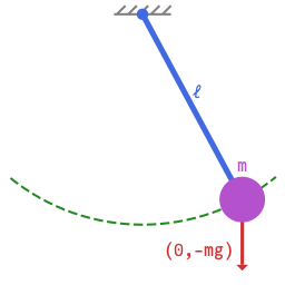
We would like to obtain a relation between the period of the swinging pendulum and the parameters we believe that are relevant to the problem.

In this case, we consider the length $\ell$ of the rod, the mass $m$ of the bob, the acceleration of gravity $g$, the angle $\theta$ of the rod with respect to the downwards vertical direction, and the period $\tau$ of the swinging pendulum.

Using Unitful.jl to define the parameters

We use PainterQubits/Unitful.jl to define the parameters mentioned above. We define most of them as Unitful.FreeUnits, except the acceleration of gravity, which is a constant and which is given as a Unitful.Quantity.

using Unitful

ℓ = u"m"
g = 9.8u"m/s^2"
m = u"g"
τ = u"s"
θ = u"NoDims"

Feeding the parameters to UnitfulBuckinghamPi.jl

In order to use UnitfulBuckingham.jl to find the adimensional groups, we use the macro @setparameters, to "register" the parameters for the package:

using UnitfulBuckinghamPi

@setparameters ℓ g m τ θ

Finding the adimensional groups with UnitfulBuckinghamPi.jl

With the parameters registered in UnitfulBuckinghamPi.jl, we find the adimensional groups with the function pi_groups():

Π = pi_groups()

2-element Vector{Expr}:
 :(g ^ (1 // 2) * ℓ ^ (-1 // 2) * τ ^ (1 // 1))
 :(θ ^ (1 // 1))

Notice the result is of type Vector{Expr}, with two elements, corresponding to the two adimensional groups obtained from the set of parameters, $\Pi = [\Pi_1, \Pi_2]$.

The last one is simply the angle $\Pi_2 = \theta$ and the first one is the sought-after adimensional relation for the period:

$$\Pi_1 = \frac{g^{1/2} \tau}{\ell^{1/2}}.$$

How does it work?

During the execution of pi_groups(), the package builds the "parameter-to-dimension" matrix, which associates each parameter to the combination of base dimensions in it:

pdmat = UnitfulBuckinghamPi.parameterdimensionmatrix()

3×5 Matrix{Rational{Int64}}:
 0  -2  0  1  0
 0   0  1  0  0
 1   1  0  0  0

Notice this is a Matrix of Rational elements. The double slash means division, for Rational elements. Rational elements are used to avoid floating point errors messing up with the powers.

The columns correspond to the parameters $\ell, g, m, τ, θ$, respectively, while the rows correspond to the dimensions $T, M, L$, standing for time, mass and length. The coefficients of the matrix are the powers of each dimension in each parameter.

The coefficients of this matrix can also be seen as the multiplicative factors in the log-log relation between the dimensions and the parameters. More precisely, let us take the length $\ell$ of the rod, whose dimension is $[\ell] = L = T^0 L^1 M^0$. Taking the logarithm of this expression, we find

$$\log[\ell] = 0 \log T + 0 \log M + 1 \log L = (0, 0, 1) \left(\begin{matrix} \log T \\ \log M \\ \log L \end{matrix}\right).$$

As for the acceleration of gravity, $g$, whose dimension is $[g] = L/T = T^{-2} L^1 M^0$, we have

$$\log[g] = -2 \log T + 0 \log M + 1 \log L = (-2, 0, 1) \left(\begin{matrix} \log T \\ \log M \\ \log L\end{matrix}\right).$$

Similarly,

$$\log[m] = 0 \log T + 1 \log M + 0 \log L = (0, 1, 0) \left(\begin{matrix} \log T \\ \log M \\ \log L \end{matrix}\right).$$ $$\log[\tau] = 1 \log T + 0 \log M + 0 \log L = (1, 0, 0) \left(\begin{matrix} \log T \\ \log M \\ \log L\end{matrix}\right).$$ $$\log[\theta] = 0 \log T + 0 \log M + 0 \log L = (0, 0, 0) \left(\begin{matrix} \log T \\ \log M \\ \log L\end{matrix}\right).$$

One can think of $\log[\ell], \log[g], \log[m], \log[\tau]$, and $\log[\theta]$ as vectors in a three-dimensional space of "dimensions", with $\{\log T, \log M, \log L\}$ being a basis for this space, and with the expressions above as the representation of those vectors in this basis.

The matrix whose rows are composed of the representation of those vectors in this basis is our "parameter-to-dimension" matrix.

Note, however, that this log-log relation is an informal way of addressing the powers of the dimensions involved in a dimensional group. The logarithm is, in principle, only defined for nondimensional quantities. We can very well arrive at the results below by working directly with the powers.

Now, the Buckingham-Pi Theorem states that

Theorem (Buckingham-Pi) Consider a system with $n$ quantities in which $m$ fundamental (base) dimensions are involved. Then, there are $n-m$ adimensional groups which can be expressed as monomials of the given quantities.

So, the adimensional groups, let's call them $\pi_1, \ldots, \pi_{n-m}$ as originally done, are found as monomials

$$\pi_j = q_1^{a^j_1}\cdots q_n^{a^j_n}, \quad j=1, \ldots, n-m.$$

By considering the dimesion of the group, and of each parameter, and taking the logarithm of the relation so obtained, we find

$$\log[\pi_j] = a^j_1\log[q_1] + \cdots + a^j_n \log[q_n], \quad \quad j=1, \ldots, n-m.$$

Since we want each $\pi_j$ to be adimensional, we require $[\pi_j] = 1$, hence $\log[\pi_j] = 0$. Therefore, we would like to solve the system

$$a^j_1\log[q_1] + \cdots + a^j_n \log[q_n] = 0, \qquad \quad j=1, \ldots, n-m.$$

The parameters have mixed dimensions, so, in order to solve the above system, we rewrite the dimension $[q_i]$ of each parameter in terms of the fundamental $m$ dimensions, say $D_1, \ldots, D_m$:

$$[q_i] = D_1^{\beta_1^i}\ldots D_m^{\beta_m^i},$$

where the $\beta_j^i$ are suitable powers for each parameter and each dimension. Taking the logarithm, we have

$$\log[q_i] = \beta_1^i \log D_1 + \ldots + \beta_m^i \log D_m.$$

Each vector $(\beta_j^i)_{j=1}^m$ forms one column of the "parameter-to-dimension" matrix mentioned above:

$$A = \left[ \begin{matrix} \beta_1^1 & \ldots & \beta_1^n \\ \vdots & & \vdots \\ \beta_m^1 & \ldots & \beta_m^n \end{matrix}\right].$$

By substituting the expression (11) for $\log[q_i]$ in the system of equations (9), we rewrite the system in matrix form

$$\left[ \begin{matrix} \beta_1^1 & \ldots & \beta_1^n \\ \vdots & & \vdots \\ \beta_m^1 & \ldots & \beta_m^n \end{matrix}\right] \left(\begin{matrix} a^j_1 \\ \vdots \\ a^j_n \end{matrix}\right) = \left(\begin{matrix} 0 \\ \vdots \\ 0 \end{matrix}\right).$$

Now it becomes clear that the solutions form the null space of the matrix $A$. If $n>m$, there are infinitely many solutions. There are, correspondingly, infinitely many adimensional groups. What we can do is to select just a few, just enough to span the whole null space. This will give us a "minimal" set of adimensional groups.

Hence, what we need is to find a basis for the null space. This may be obtained in several ways, by factoring $A$ in one of many forms, such as QR, LU, SVG, and so on.

However, since we want to preserve the Rational type of the elements of the "parameter-to-dimension" matrix, we choose to perform an LU factorization of the matrix $A$. In doing so, we find the null space of $A$ by looking for the null space of $U$.

Of course, any decent computer language used in Scientific Computing has implementation for several different factorizations. The difficulty, however, is to find one that supports Rational types and for which the LU decomposition preserves this type. Such an LU factorization is available in the standard LinearAlgebra package of the Julia programming language.

The only problem, however, is that this implementation of the LU factorization does not include full pivoting, only row pivoting. This means the factorization may fail when the matrix is singular and needs column pivoting.

In order to overcome this problem, we implement, in UnitfulBuckinghamPi.jl, our own LU factorization, with full pivoting. And we take care of preserving the eltype of the matrix $A$.

The full pivoting algorithm yields two permutation vectors $\vec{p}$ and $\vec{q}$, a square $m\times m$ lower-triangular matrix $L$, and an upper-triangular $m\times n$ matrix $U$ such that $LU = PAQ,$ where $P$ and $Q$ are the permutation matrices associated with the permutation vectors $\vec{p}$ and $\vec{q}$. In Julia vector/matrix notation, this is the same as L*U = A[p;q].

Going back to the matrix pdmat obtained for the simple pendulum problem above, we perform the factorization

L, U, p, q = UnitfulBuckinghamPi.lu_pq(pdmat)

Then, we obtain the matrix L:

3×3 Matrix{Rational{Int64}}:
   1    0  0
 -1//2  1  0
   0    0  1

The matrix U:

3×5 Matrix{Rational{Int64}}:
 -2  0  0   1    0
  0  1  0  1//2  0
  0  0  1   0    0

The permutation vector p:

3-element Vector{Int64}:
 1
 3
 2

And the permutation vector q:

5-element Vector{Int64}:
 2
 1
 3
 4
 5

By looking at the matrix U, we see that the first three columns are linearly independent, while column four is a linear combination of the first two and the fifth column is plain zero. Hence, U has full rank three, and null space with dimension two. We may find a basis $\{\vec{v}_\alpha, \vec{v}_\beta\}$ for the null space by solving $U\vec{v} = 0$ with $\vec{v} = \vec{v}_\alpha$ of the form $\vec{v}_\alpha = (v_1,v_2,v_3,1,0)$ and $\vec{v} = \vec{v}_\beta$ of the form $\vec{v}_\beta = (v_1, v_2, v_3, 0, 1)$.

Hence, we solve

$$\left[ \begin{matrix} -2 & 0 & 0 \\ 0 & 1 & 0 \\ 0 & 0 & 1 \end{matrix}\right] \left(\begin{matrix} v_1 \\ v_2 \\ v_3 \end{matrix} \right) = - \left(\begin{matrix} 1 \\ 1/2 \\ 0 \end{matrix}\right),$$

to find $\vec{v}_\alpha = (1/2, -1/2, 0, 1, 0)$, and we solve

$$\left[ \begin{matrix} -2 & 0 & 0 \\ 0 & 1 & 0 \\ 0 & 0 & 1 \end{matrix}\right] \left(\begin{matrix} v_1 \\ v_2 \\ v_3 \end{matrix} \right) = - \left(\begin{matrix} 0 \\ 0 \\ 0 \end{matrix}\right),$$

to find $\vec{v}_\beta = (0, 0, 0, 0, 1)$.

Let us not forget that the columns have been permuted according to the vector $\vec{q} = (2,1,3,4,5)$. Hence, the columns, which originally corresponded to the (logarithm of the dimension of the) parameters $ℓ, g, m, τ, θ$, now correspond to (idem) $g, ℓ, m, τ, θ$, respectively. Then, taking this into consideration, equation (9), in this case, takes the form

$$(1/2) \log[g] + (-1/2) \log[\ell] + (0)\log[m] + (1)\log[\tau] + (0)\log[\theta] = 0$$

and

$$(0) \log[g] + (0) \log[\ell] + (0)\log[m] + (0)\log[\tau] + (1)\log[\theta] = 0.$$

Rewriting them, we have

$$(1/2) \log[g] + (-1/2) \log[\ell] + (1)\log[\tau] = 0, \qquad \log[\theta] = 0.$$

Exponentiating them, we finally obtain the two adimensional groups

$$\Pi_1 = \frac{g^{1/2}\tau}{\ell^{1/2}}, \qquad \Pi_2 = \theta.$$

This concludes the analysis.